10GbE Media Converters transparently connect 10 Gigabit Ethernet links over multimode or single mode fiber. Each 10G Media Converter comes with pluggable transceiver ports that support fiber to fiber, copper to fiber or copper to copper media conversion.10G media converter are complete and versatile solutions for the application such as FTTx, CWDM and carrier Ethernet. By the diversified speeds of 1,000Mbps and 10G, N-net provides standalone 10G media converter products for different applications and can be applied as per your ideal network topology. 10G Fiber Media Converter,Fiber Optic Media Converter,Fiber Optic Converter,Fiber Media Converter Shenzhen N-net High-Tech Co.,Ltd , http://www.nnetswitch.com
IntroductionLFSRs (linear feedback shift registers) provide a simple means for generating nonsequential lists of numbers quickly on microcontrollers. Generating the pseudo-random numbers only requires a right-shift operation and an XOR operation. Figure 1 shows a 5-bit LFSR. Figure 2 shows an LFSR implementation in C, and Figure 3 shows a 16-bit LFSR implementation in 8051 assembly.
LFSRs and polynomialsA LFSR is specified entirely by its polynomial. For example, a 6th-degree polynomial with every term present is represented with the equation x6 + x5 + x4 + x3 + x2 + x + 1. There are 2 (6-1) = 32 different possible polynomials of this size. Just as with numbers, some polynomials are prime or primitive. We are interested in primitive polynomials because they will give us maximum length periods when shifting. A maximum length polynomial of degree n will have 2n-1 different states. A new state is transitioned to after each shift. Consequently, a 6th-degree polynomial will have 31 different states. Every number between 1 and 31 will occur in the shift register before it repeats. In the case of primitive 6th-degree polynomials, there are only six. Table 1 lists all the primitive 6th-degree polynomials and their respective polynomial masks. The polynomial mask is created by taking the binary representation of the polynomial and truncating the right-most bit. The mask is used in the code that implements the polynomial. It takes n bits to implement the polynomial mask for an nth-degree polynomial.
Every primitive polynomial will have an odd number of terms, which means that every mask for a primitive polynomial will have an even number of 1 bit. Every primitive polynomial also defines a second primitive polynomial, its dual. The dual can be found by subtracting the exponent from the degree of the polynomial for each term. For example, given the 6th-degree polynomial, x6 + x + 1, its dual is x6-6 + x6-1 + x6-0, which is equal to x6 + x5 + 1. In Table 1, polynomials 1 and 2, 3 and 4, 5 and 6 are the duals of each other.
Table 2 lists the period of each different size polynomial and the number of primitive polynomials that exist for each size. Table 3 lists one polynomial mask for each polynomial of a different size. It also shows the first four values ​​that the LFSR will hold after consecutive shifts when the LFSR is initialized to one. This table should help to ensure that the implementation is correct.
The structure of a LFSR LFSRs can never have the value of zero, since every shift of a zeroed LFSR will leave it as zero. The LFSR must be initialized, ie, seeded, to a nonzero value. When the LFSR holds 1 and is shifted once, its value will always be the value of the polynomial mask. When the register is all zeros except the most significant bit, then the next several shifts will show the high bit shift to the low bit with zero fill. For example, any 8 -bit shift register with a primitive polynomial will eventually generate the sequence 0x80, 0x40, 0x20, 0x10, 8, 4, 2, 1 and then the polynomial mask.
Generating pseudo-random numbers with LFSRIn general, a basic LFSR does not produce very good random numbers. A better sequence of numbers can be improved by picking a larger LFSR and using the lower bits for the random number. For example, if you have a 10-bit LFSR and want an 8-bit number, you can take the bottom 8 bits of the register for your number. With this method you will see each 8-bit number four times and zero, three times, before the LFSR finishes one period and repeats. This solves the problem of getting zeros, but still the numbers do not exhibit very good statistical properties. Instead you can use a subset of the LFSR for a random number to increase the permutations of the numbers and improve the random properties of the LFSR output.
Shifting the LFSR more than once before getting a random number also improves its statistical properties. Shifting the LFSR by a factor of its period will reduce the total period length by that factor. Table 2 has the factors of the periods.
The relatively short periods of the LFSRs can be solved by XORing the values ​​of two or more different sized LFSRs together. The new period of these XORed LFSRs will be the LCM (least common multiple) of the periods. For example, the LCM of a primitive 4-bit and a primitive 6-bit LFSR is the LCM (15, 63), which is 315. When joining LFSRs in this way, be sure to use only the minimum number of bits of the LFSRs; it is a better practice to use less than that. With the 4- and 6-bit LFSRs, no more than the bottom 4 bits should be used. In Figure 2, the bottom 16 bits are used from 32- and 31-bit LFSRs. Note that XORing two LFSRs of the same size will not increase the period.
The unpredictability of the LFSRs can be increased by XORing a bit of "entropy" with the feedback term. Some care should be taken when doing this—there is a small chance that the LFSR will go to all zeros with the addition of the entropy bit . The zeroing of the LFSR will correct itself if entropy is added periodically. This method of XORing a bit with the feedback term is how CRCs (cyclic redundancy checks) are calculated.
Polynomials are not created equal. Some polynomials will definitely be better than others. Table 2 lists the number of primitive polynomials available for bit sizes up to 31 bits. Try different polynomials until you find one that meets your needs. The masks given in Table 3 were randomly selected.
All the basic statistical tests used for testing random number generators can be found in Donald Knuths, The Art of Computer Programming, Volume 2, Section 3.3. More extensive testing can be done using NIST's Statistical Test Suite. NIST also has several publications describing random number testing and references to other test software. 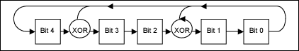
Figure 1. Simplified drawing of a LFSR. 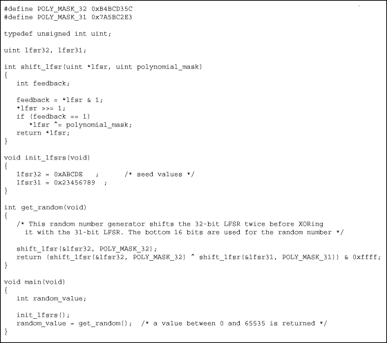
Figure 2. C code implementing a LFSR. 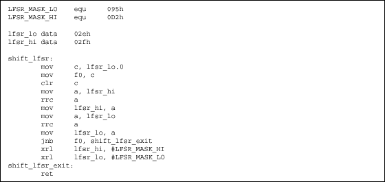
Figure 3. 8051 assembly code to implement a 16-bit LFSR with mask 0D295h.
Table 1. All 6th-degree primitive polynomials Irreducible Polynomial In Binary Form Binary Mask Mask 1 x6 + x + 1 1000011b 100001b 0x21 2 x6 + x5 + 1 1100001b 110000b 0x30 3 x6 + x5 + x2 + x + 1 1100111b 110011b 0x33 4 x6 + x5 + x4 + x + 1 1110011b 111001b 0x39 5 x6 + x5 + x3 + x2 + 1 1101101b 110110b 0x36 6 x6 + x4 + x3 + x + 1 1011011b 101101b 0x2D
Table 2. Polynomial information Degree Period Factors of Period No. of Primitive Polynomials of This Degree 3 7 7 2 4 15 3, 5 2 5 31 31 6 6 63 3, 3, 7 6 7 127 127 18 8 255 3, 5, 17 16 9 511 7, 73 48 10 1,023 3, 11, 31 60 11 2,047 23, 89 176 12 4,095 3, 3, 5, 7, 13 144 13 8,191 8191 630 14 16,383 3, 43, 127 756 15 32,767 7, 31, 151 1,800 16 65,535 3, 5, 17, 257 2,048 17 131,071 131071 7,710 18 262,143 3, 3, 3, 7, 19, 73 7,776 19 524,287 524287 27,594 20 1,048,575 3, 5, 5, 11, 31, 41 24,000 twenty one 2,097,151 7, 7, 127, 337 84,672 twenty two 4,194,303 3, 23, 89, 683 120,032 twenty three 8,388,607 47, 178481 356,960 twenty four 16,777,215 3, 3, 5, 7, 13, 17, 241 276,480 25 33,554,431 31, 601, 1801 1,296,000 26 67,108,863 3, 2731, 8191 1,719,900 27 134,217,727 7, 73, 262657 4,202,496 28 268,435,455 3, 5 29, 43, 113, 127 4,741,632 29 536,870,911 233, 1103, 2089 18,407,808 30 1,073,741,823 3, 3, 7, 11, 31, 151, 331 17,820,000 31 2,147,483,647 2147483647 69,273,666 32 4,294,967,295 3, 5, 17, 257, 65537 Not Available
Table 3. Sample masks and first four values ​​output after initializing LFSR with one Degree Typical Mask First Four Values ​​in LFSR After Consecutive Shifts 3 0x5 0x5 0x7 0x6 0x3 4 0x9 0x9 0xD 0xF 0xE 5 0x1D 0x1D 0x13 0x14 0xA 6 0x36 0x36 0x1B 0x3B 0x2B 7 0x69 0x69 0x5D 0x47 0x4A 8 0xA6 0xA6 0x53 0x8F 0xE1 9 0x17C 0x17C 0xBE 0x5F 0x153 10 0x32D 0x32D 0x2BB 0x270 0x138 11 0x4F2 0x4F2 0x279 0x5CE 0x2E7 12 0xD34 0xD34 0x69A 0x34D 0xC92 13 0x1349 0x1349 0x1AED 0x1E3F 0x1C56 14 0x2532 0x2532 0x1299 0x2C7E 0x163F 15 0x6699 0x6699 0x55D5 0x4C73 0x40A0 16 0xD295 0xD295 0xBBDF 0x8F7A 0x47BD 17 0x12933 0x12933 0x1BDAA 0xDED5 0x14659 18 0x2C93E 0x2C93E 0x1649F 0x27B71 0x3F486 19 0x593CA 0x593CA 0x2C9E5 0x4F738 0x27B9C 20 0xAFF95 0xAFF95 0xF805F 0xD3FBA 0x69FDD twenty one 0x12B6BC 0x12B6BC 0x95B5E 0x4ADAF 0x10E06B twenty two 0x2E652E 0x2E652E 0x173297 0x25FC65 0x3C9B1C twenty three 0x5373D6 0x5373D6 0x29B9EB 0x47AF23 0x70A447 twenty four 0x9CCDAE 0x9CCDAE 0x4E66D7 0xBBFEC5 0xC132CC 25 0x12BA74D 0x12BA74D 0x1BE74EB 0x1F49D38 0xFA4E9C 26 0x36CD5A7 0x36CD5A7 0x2DABF74 0x16D5FBA 0xB6AFDD 27 0x4E5D793 0x4E5D793 0x6973C5A 0x34B9E2D 0x5401885 28 0xF5CDE95 0xF5CDE95 0x8F2B1DF 0xB25867A 0x592C33D 29 0x1A4E6FF2 0x1A4E6FF2 0xD2737F9 0x1CDDF40E 0xE6EFA07 30 0x29D1E9EB 0x29D1E9EB 0x3D391D1E 0x1E9C8E8F 0x269FAEAC 31 0x7A5BC2E3 0x7A5BC2E3 0x47762392 0x23BB11C9 0x6B864A07 32 0xB4BCD35C 0xB4BCD35C 0x5A5E69AE 0x2D2F34D7 0xA22B4937
N-net 10G media converter supports various interfaces such as UTP, SFP, SFP+, XFP etc. All these interfaces are developed to support the protocols such as 100Base-Tx, 1000Base-T, 10GBase-T, and 10GBase-LR, 10GBase-SR, which makes your network more complete and solid.
Linear feedback shift registers are introduced along with the polynomials that completely describe them. The applicaTIon note describes how they can be implemented and techniques that can be used to improve the staTIsTIcal properTIes of the numbers generated.