How to Realize a Compact Visual Big Data Analysis System

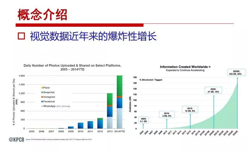
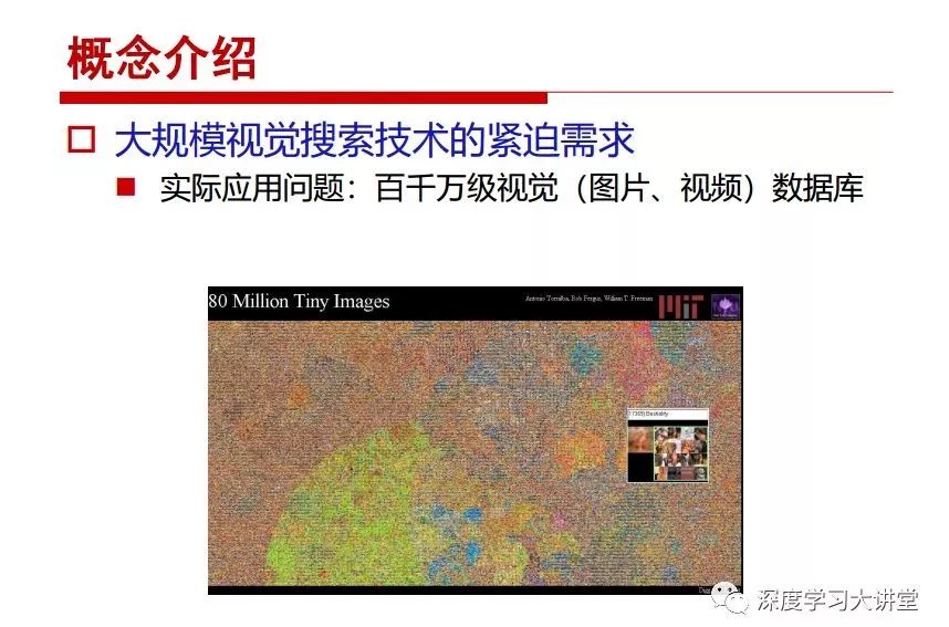
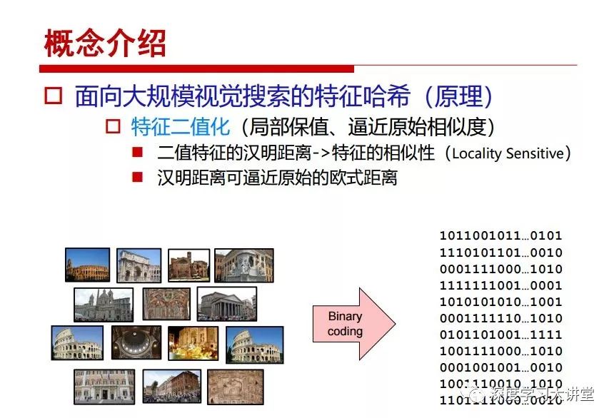
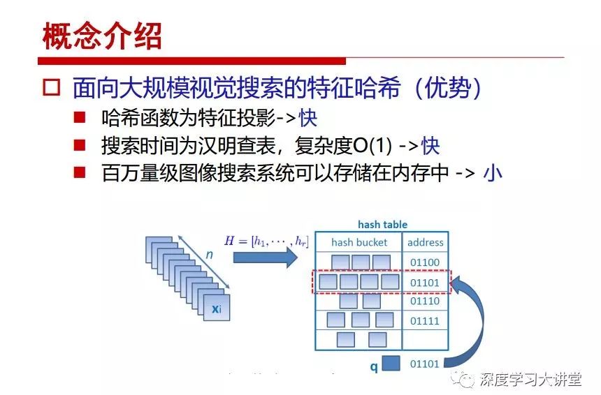
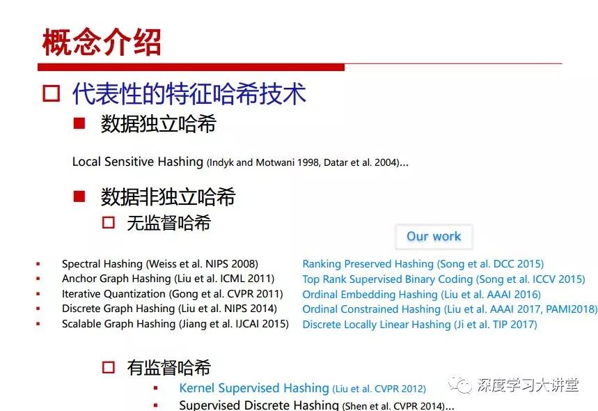
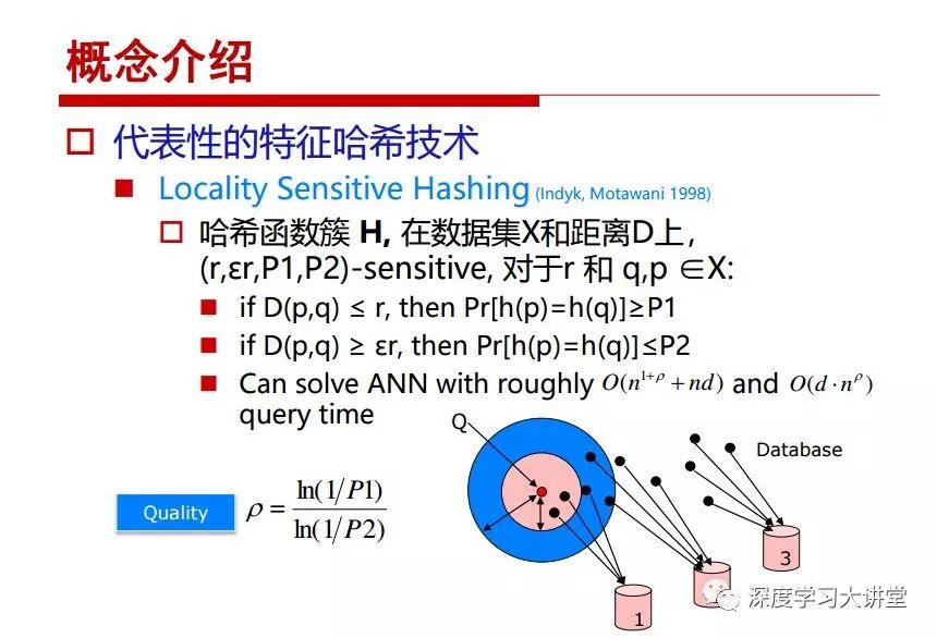
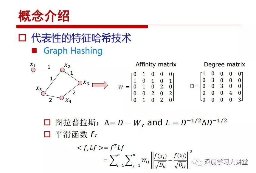
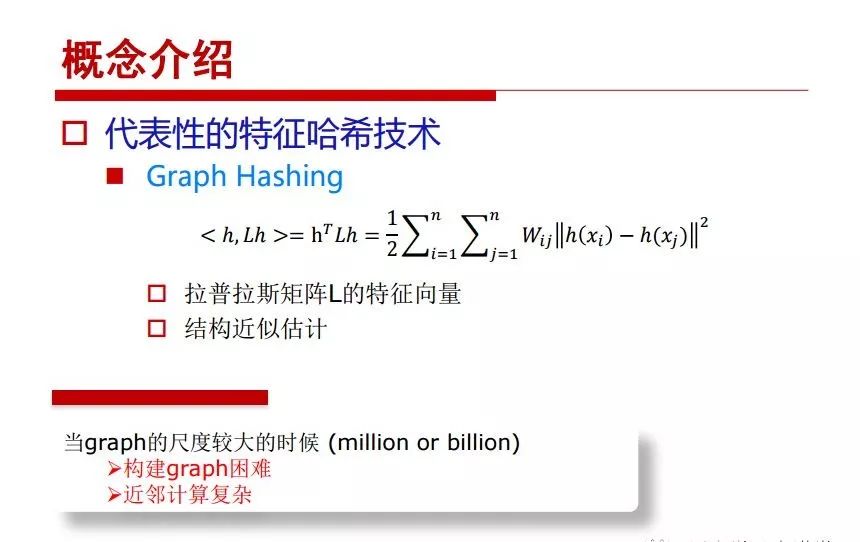
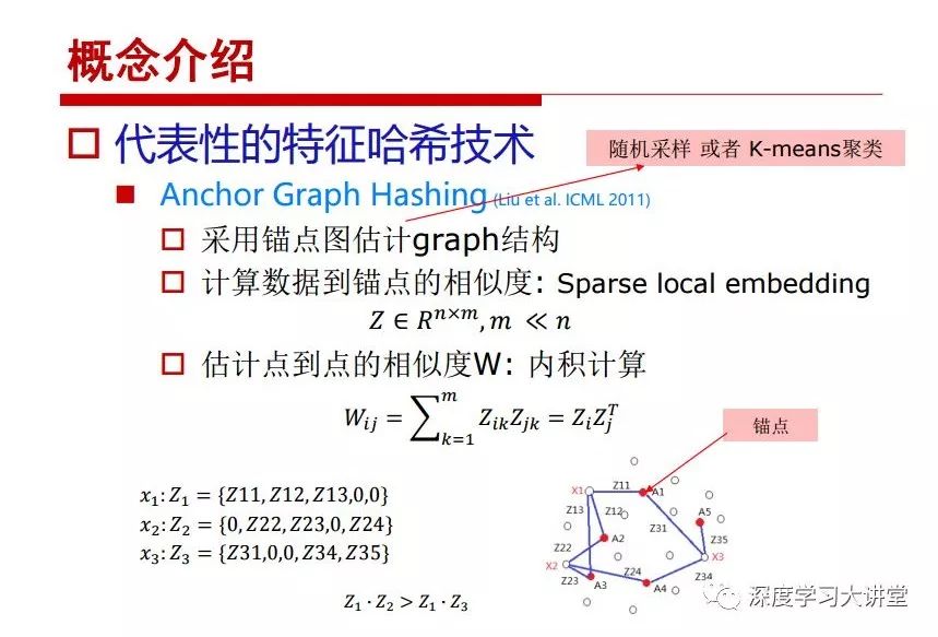
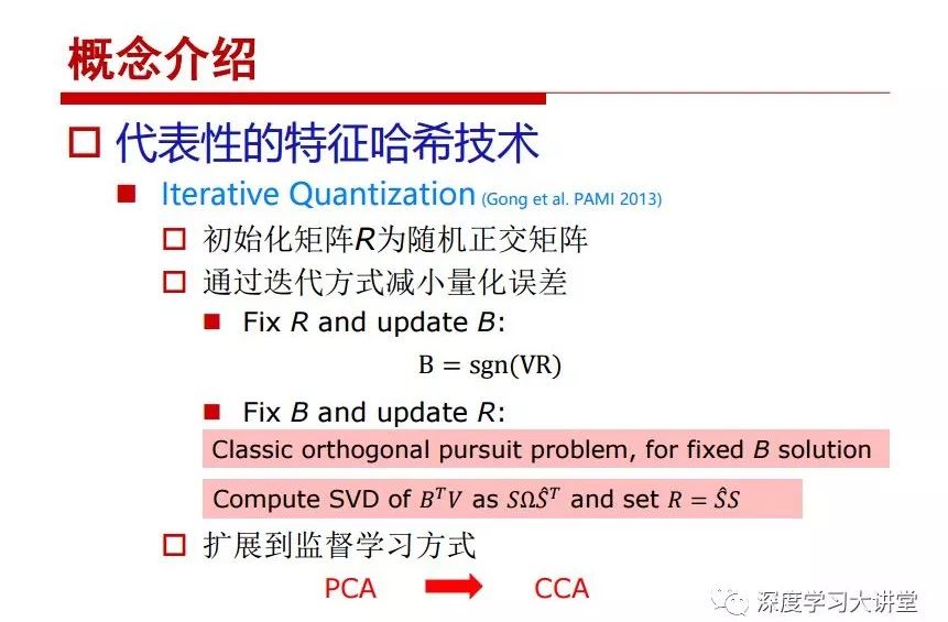
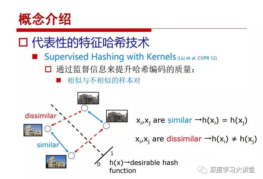
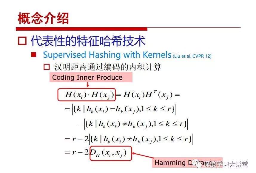
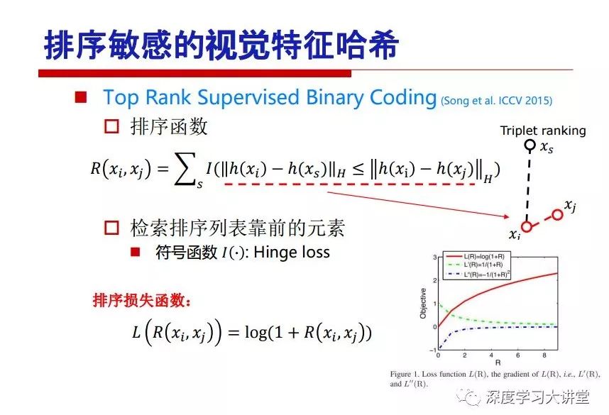
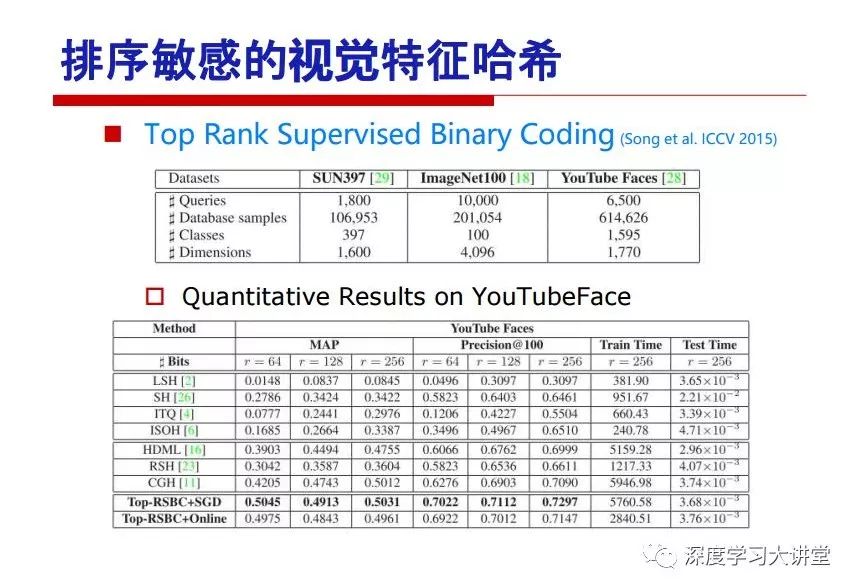
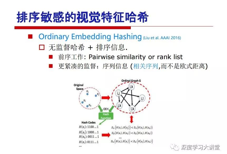
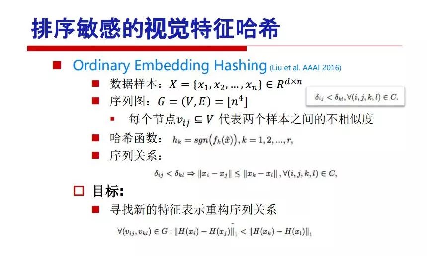
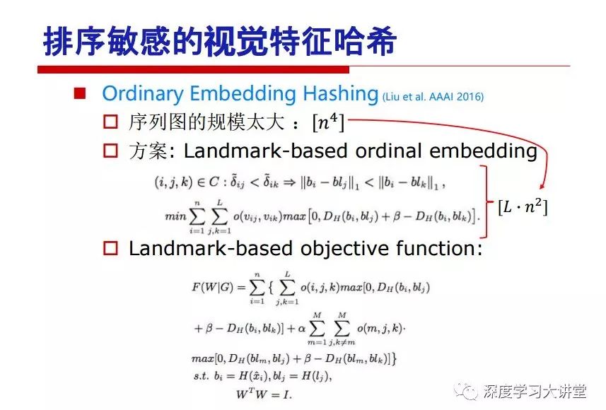
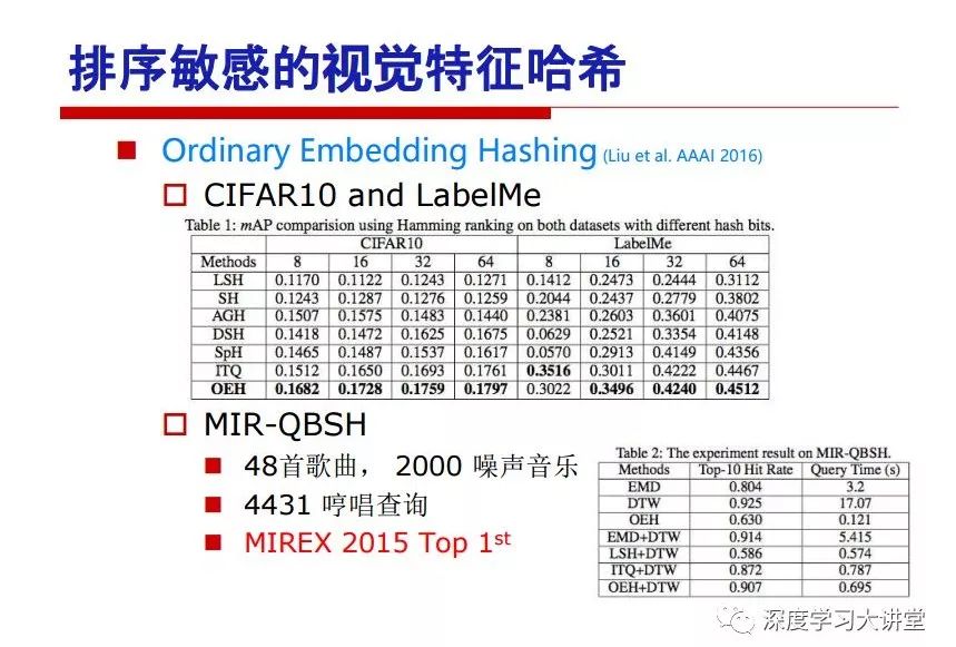
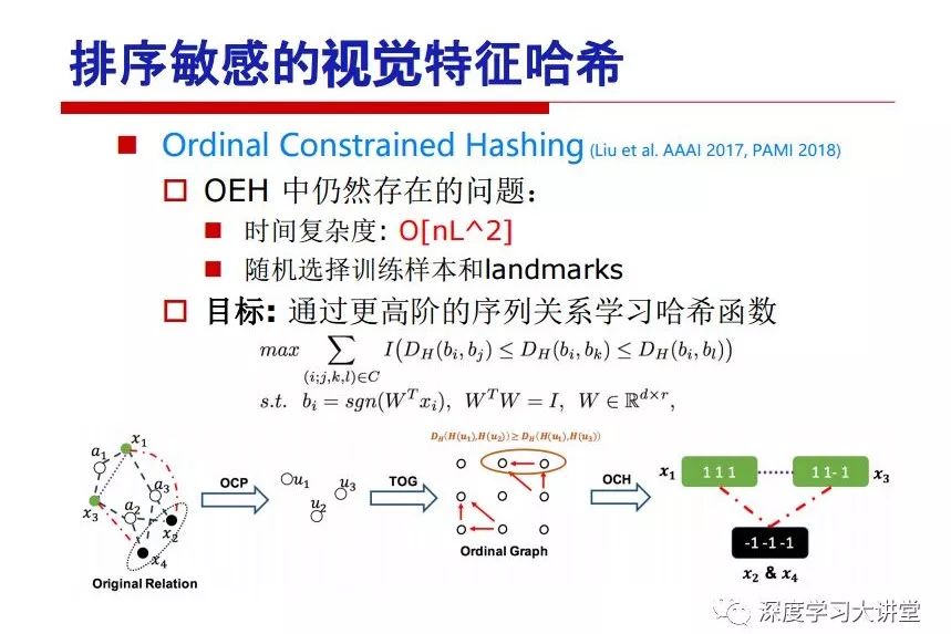
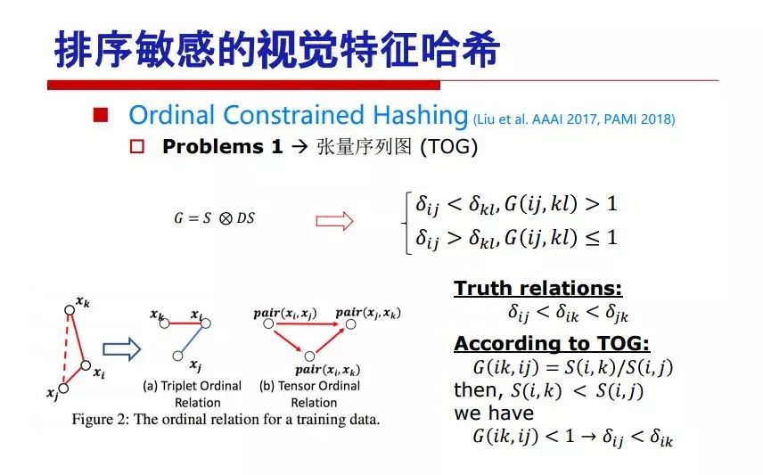
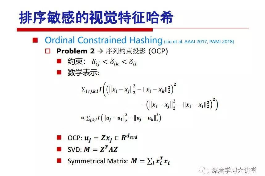
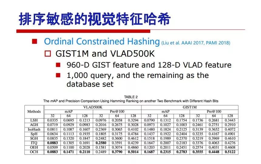
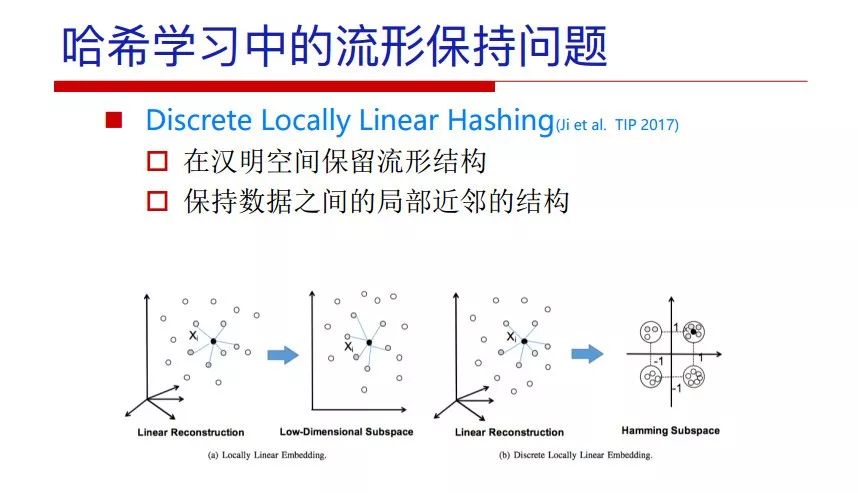
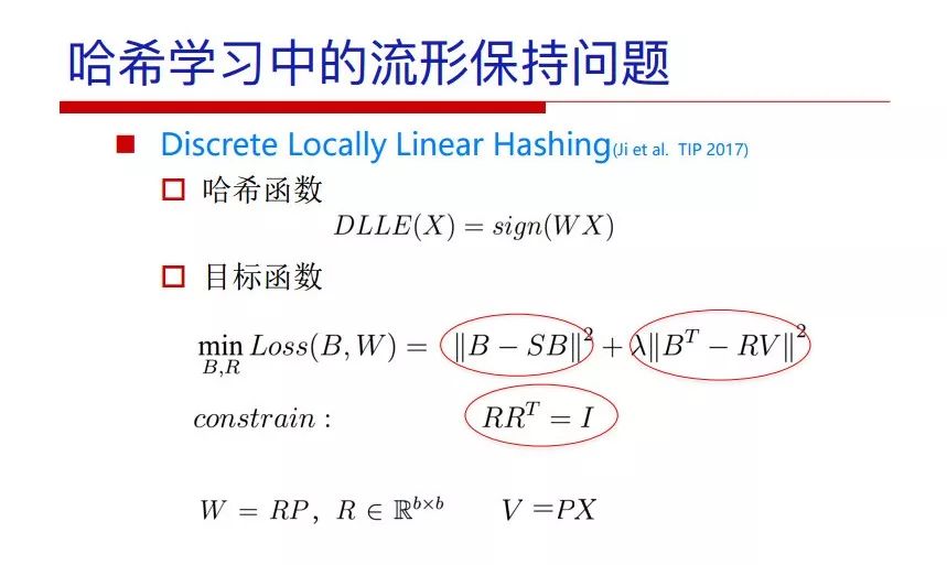
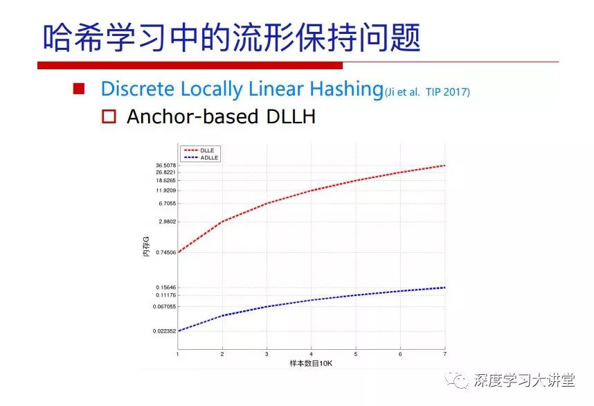
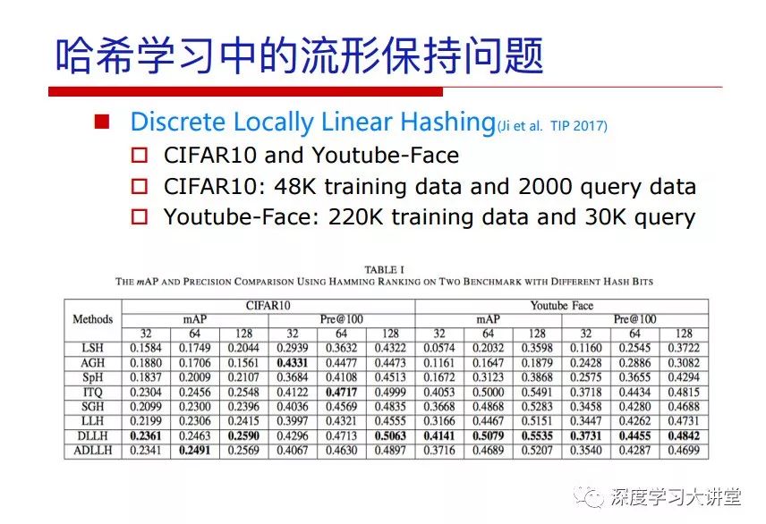
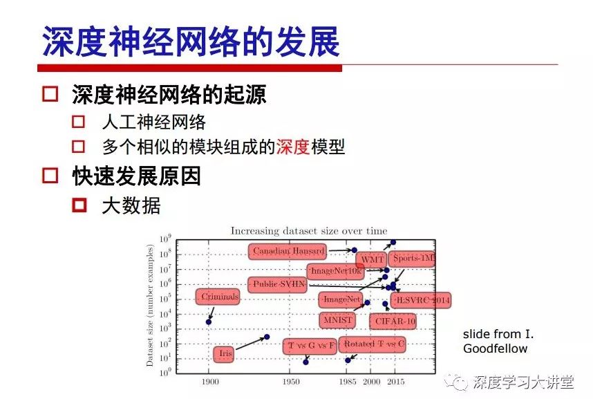
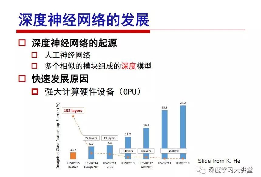
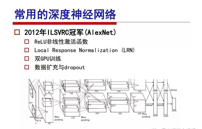
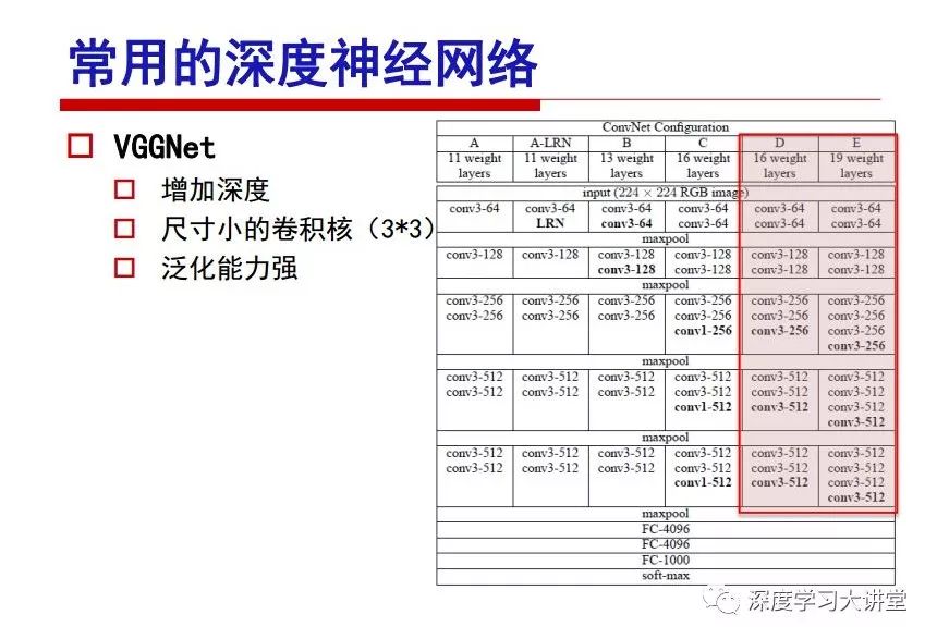
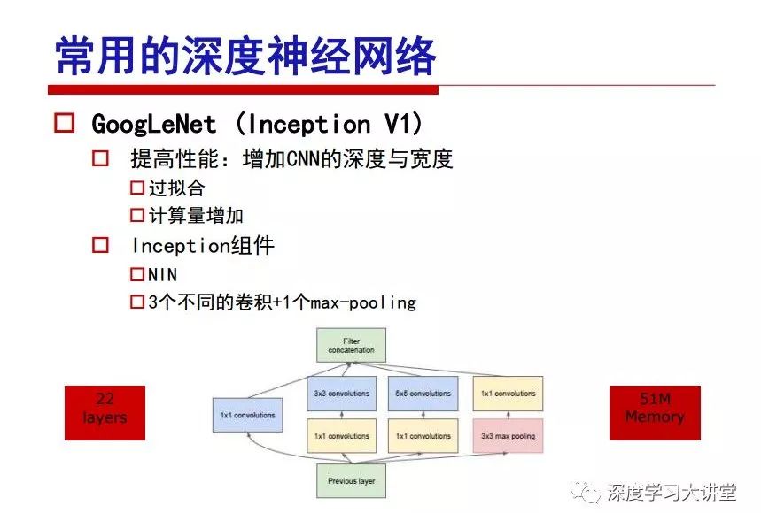
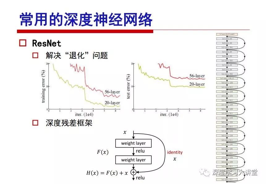
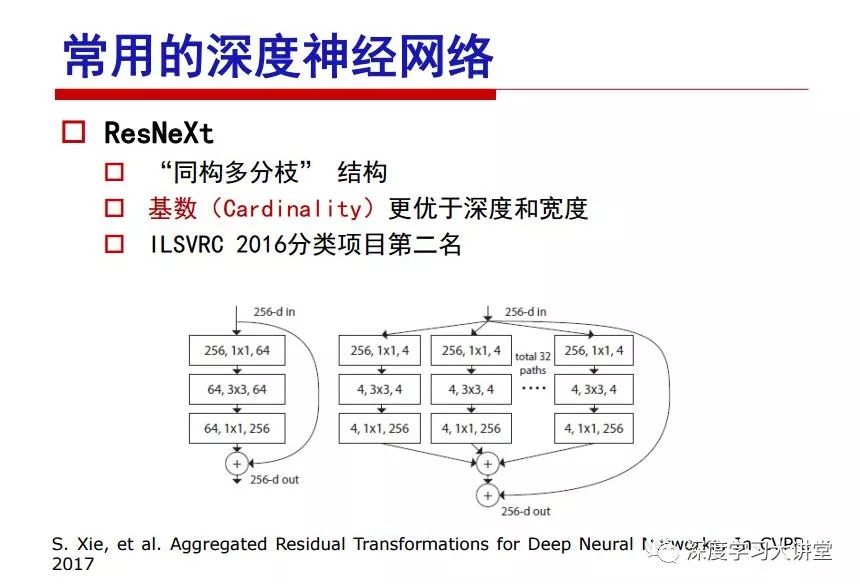
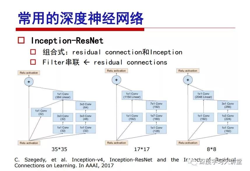
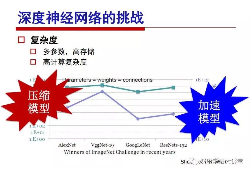
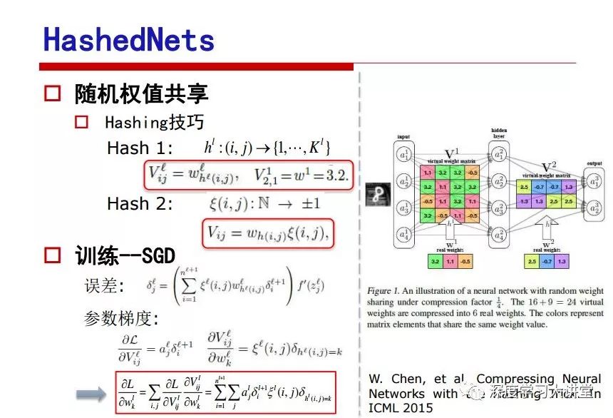
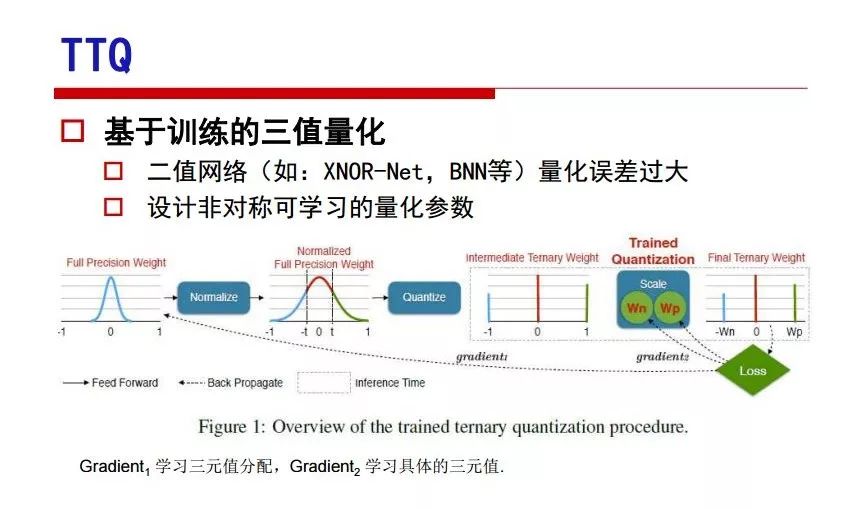
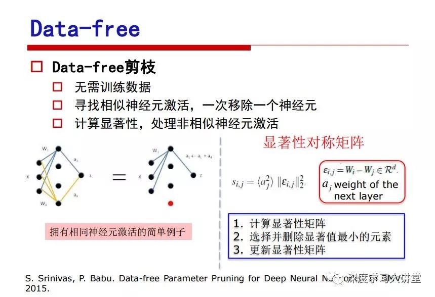
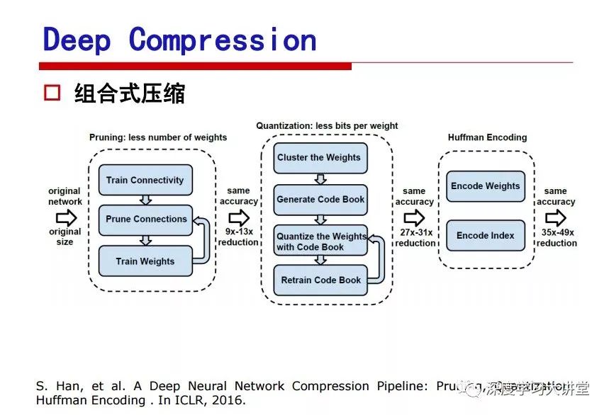
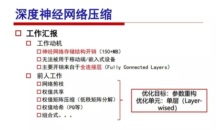
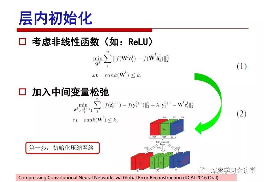
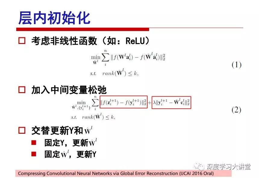
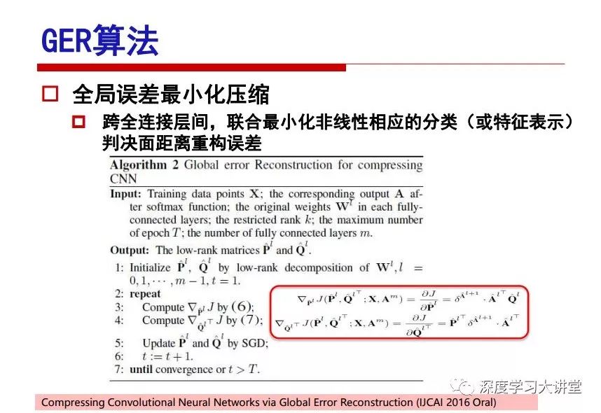
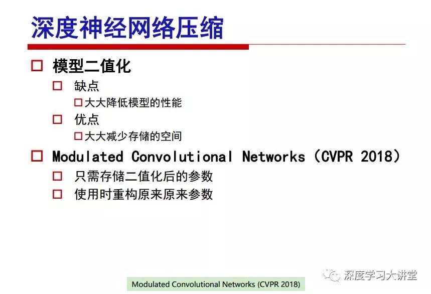
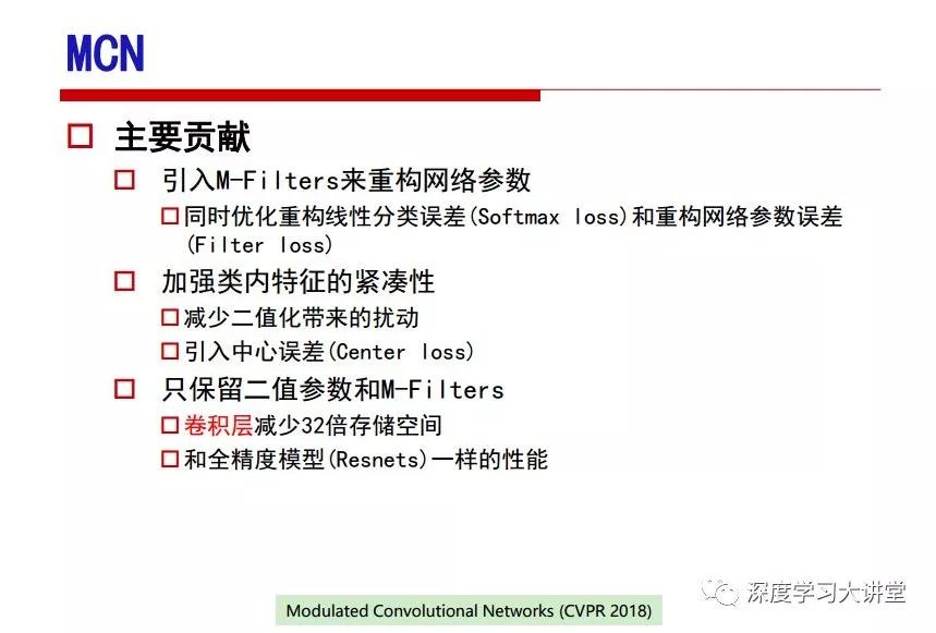
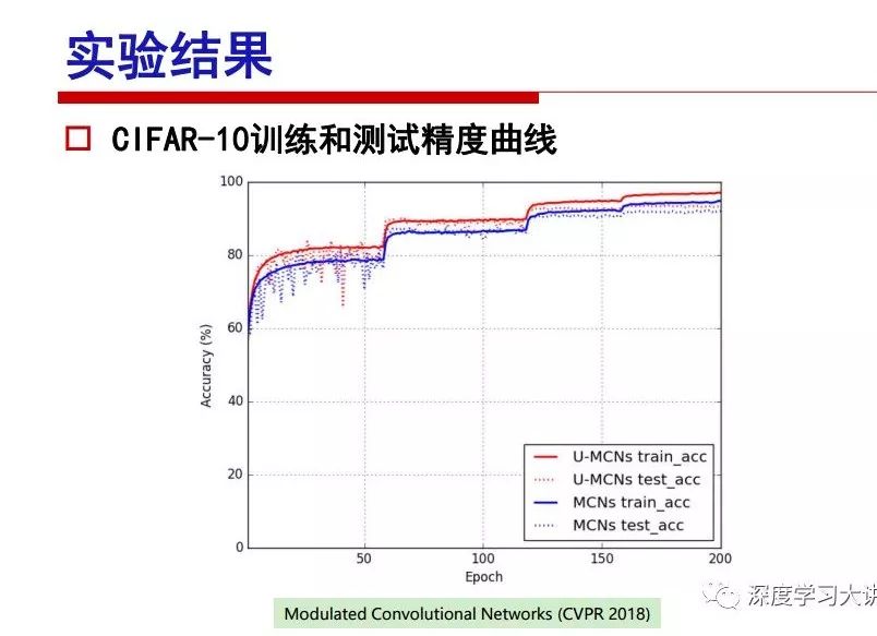
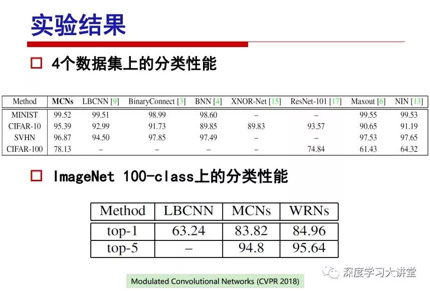
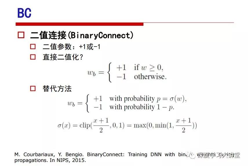
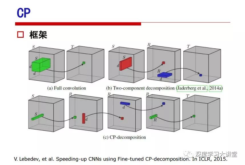
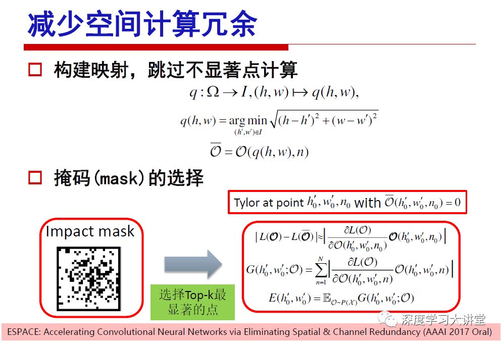
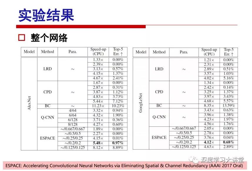
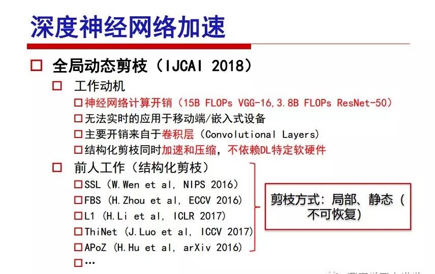
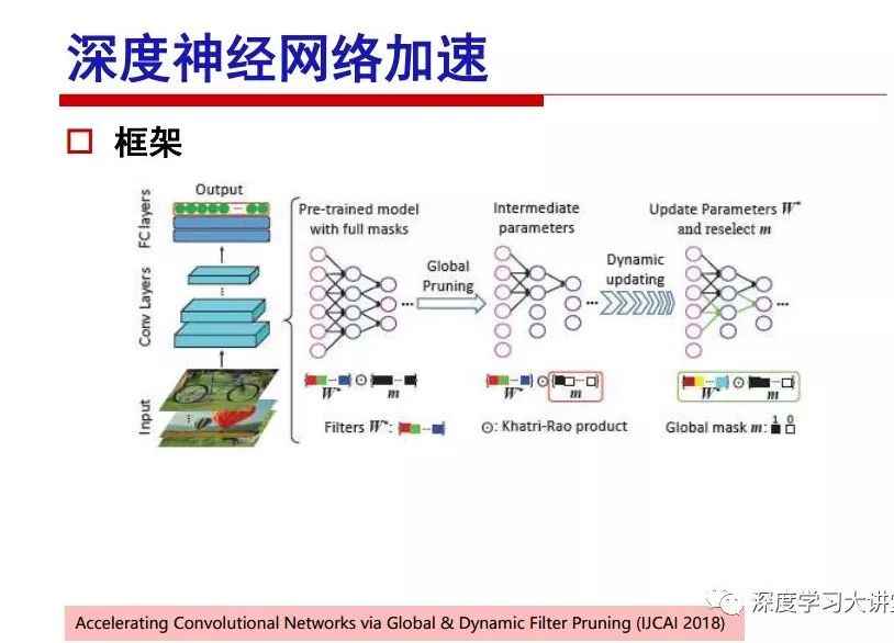
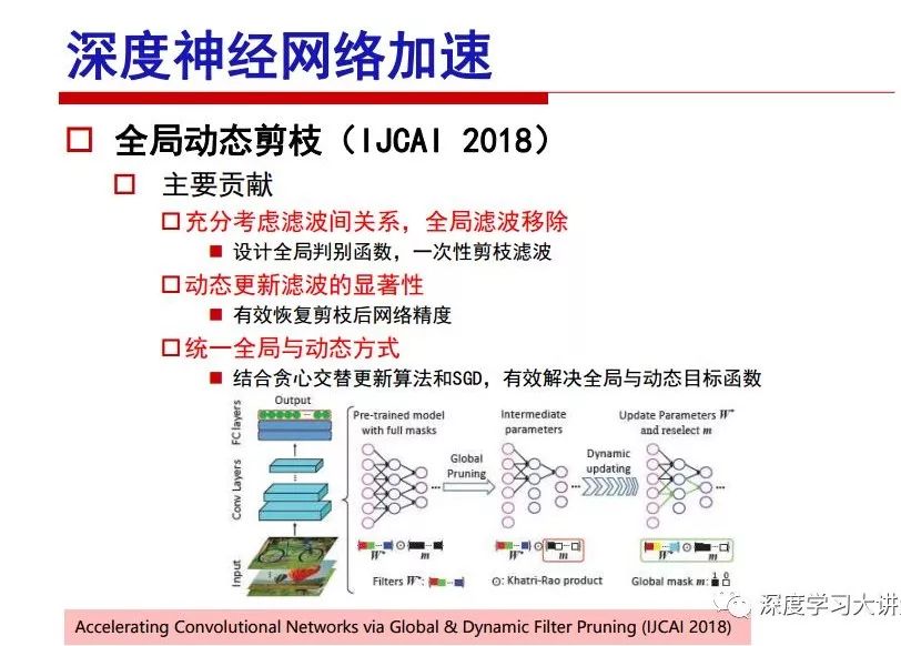
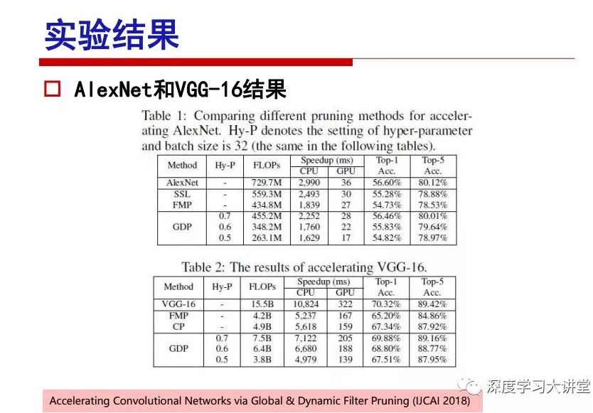
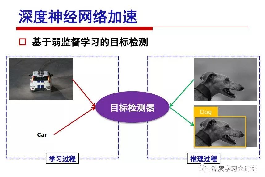
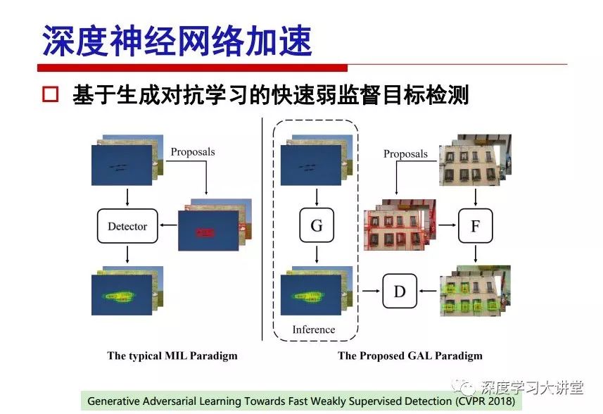
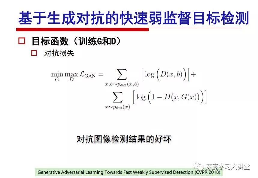
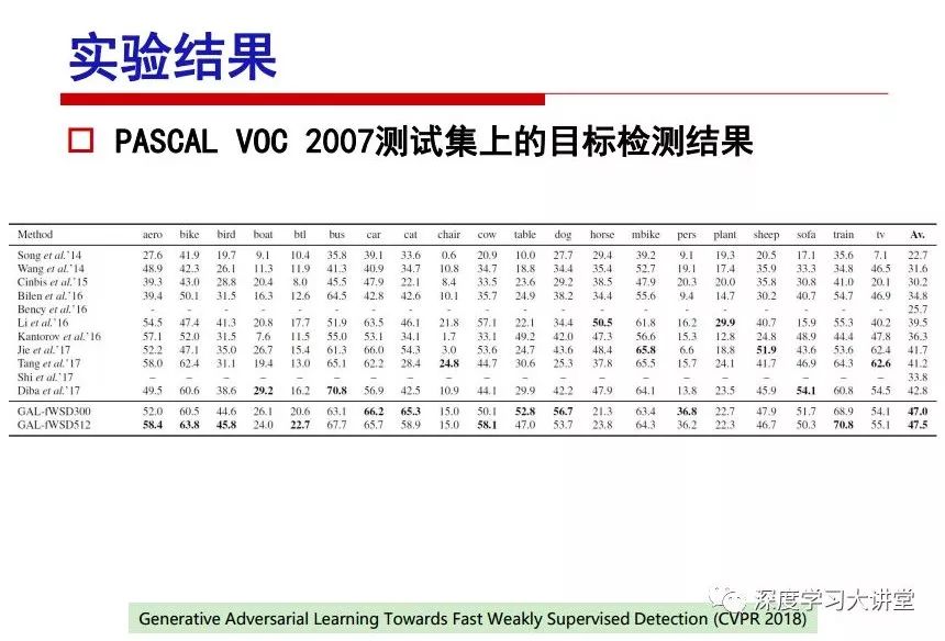
"Falling clouds and solitary flock fly together, Qiushui total long sky color."

With just fourteen words, it has abstracted the beauty of color, dynamic beauty, imaginary beauty, and three-dimensional beauty in the visual image in an extremely hierarchical manner. Therefore, it has become a must-see for landscape descriptions.

In the field of computer vision, the fourteen-character creation process is actually a process of extracting key features from the visual system and presenting them in a compact and compact manner.

Computer vision technology has faced greater computational pressure since its birth. Research in this field has also been alternating between space-for-time or time-for-space. So far, although the computing power has been greatly improved with the GPU, however, in the human-computer interaction in the real scene, there is still the problem of insufficient resources on the side. Therefore, if our feature extraction process can achieve “outline” of the entire visual input, ie, the extraction process is faster and the feature representation is more compact, it will contribute to the real landing of computer vision in life.

Today, Professor Ji Rongji from Xiamen University will introduce a compact visual big data analysis system from three aspects: the compactness of visual information, the compactness of deep networks, and the compactness of detection algorithms.

At the end of the article, the lecture hall provided the download link for references mentioned in the article.

First, brush a wave of welfare, Xiamen University Media Analysis and Computing Group, enrolling masters, doctoral students, postdoctoral, assistant professors and so on.

How can a small research group at Xiamen University do something different from others? We start from thinking about the problems of existing algorithms and think about what else is wrong with accuracy. In fact, if you look at the process of visual search and recognition, from feature extraction, description, to indexing, there are important requirements for system compactness. Although it has not caused widespread concern, there are many industrial applications. Therefore, from 2013 to now almost five years, I mainly study how to make the search system and the identification system small and fast.

This report contains three parts:

The first part is compact visual features: if the feature is drawn out without a clear target for visual feature retrieval, then how to make the feature small and fast.

The second part is the compactness of the neural network: There are many end-to-end learnings now, and how does the neural network make it faster?

The third part is the compactness of the detection algorithm.

In terms of compact visual features, visual data is the main body of big data. When it comes to big data, the first thing that comes to our attention is the image and video data.

If you can't find image and video data, their value is actually difficult to find. The problem we face this time is that we need to find relevant visual data at high speed and efficiency in millions or millions of data sets. This problem is not so easy in itself, because it is unstructured. At this time, we must use the approximate search method to find visual data at a high speed with limited loss of precision.

In order to do this, some features can now achieve the purpose of visual search, but there is no way to do it in mobile visual zooming or high-throughput search. For example, visual bag features, CNN features, and VLAD features are relatively high. In addition, some inverted indexing techniques can be used to exchange time with space. Of course, if the space overhead is too large, it can also result in movement. Problem that can't be used in either the embedded system or the embedded system.

In the past four years, my research interests have turned to the binarization of features. Given a set of image databases, we want to map each image into a binary code. If the two images are similar, it is expected that the binary code will be similar. If they are not similar, the longer the binary coded distance is, the better.

If we can achieve this goal, of course, better, we can do high-speed and efficient matching. Firstly, the feature of the hash function is projected fast. Second, his search time is Hanming's lookup table, and the complexity O(1) time is also fast. The final mega-level image can be stored in memory like a search system, making it relatively small.

Its features can be quickly and compactly stored in memory. This speed increase will bring about loss of accuracy. Therefore, after raising this question for the first time in 2004, everyone was concerned about how to reduce the loss. From the research method can be divided into two categories, the first type is the loss of the construction loss is not related to the data called data independent hash, the second is expected to consider the data distribution to the quantization error, according to the label and No label is divided into two categories, unsupervised or supervised, and it is better to have supervision, but manual labeling is very expensive. Here are some of the early published related articles.

For the stochastic partitioning of the feature space, we can ensure that if the two points are close within the original space, there is a certain probability that the generated binary space is still near. This probability is positively related to the degree of the hash bit code.

The original space is not perfect, you can create a neighbor graph for the current data set, and then go to Laplacian of the graph, hoping to get the similarity in the graph to get the binary code learning process, it is directly equivalent to adding a Weight matrix.

However, if you do this, there will be some problems. The main problem is to do Laplacian for these data and to find the eigenvectors of the matrix. We know that it is very difficult to find the matrix's feature decomposition when the matrix is ​​large.

In order to solve this problem, the use of anchor graphs to estimate the graph structure was proposed in ICML in 2011. Therefore, the similarity between data points and data points was calculated and the similarities between data points and anchor points were changed. The anchor points were then used to calculate data points. Similarity.

If we want to calculate the approximation of the matrix estimate, first we must give some constraints. We can quickly find the similar point matrix based on the anchor point through matrix decomposition, so we can speed up the calculation.

In addition, the original space is not perfect, so you can first do a PCA projection of the space, calculate the projection matrix, and then calculate the rotation matrix, by quantifying the alternating and overlapping between the two methods, which is an unsupervised method.

In addition, the supervised approach has also been involved since 2012. This is an article we wrote on CVPR. Apart from the introduction of image points between hashes, we hope that some images will be as close as possible, and some images will not Similar is better.

At that time we made a very important contribution. We calculated the Hamming distance through the inner product of the code and proved it through mathematical calculations. Since then, it has developed rapidly. We have also done a lot of work.

Today mainly introduces two aspects. The first inception of 2015 was to sort the hash of sensitive visual features and how to embed the sort information into the learning of binary codes during the hash learning process. The second aspect is how to do graphic processing in the binary learning space. The first motive was first published on the 2015 ICCV. The previous job was Pairwise similarity. We want to make a hash feature, its purpose is to do the search. The sorting information you get is more from its ranking list. So we expect that if there is an original ranking in the feature space, we hope to map it to a binary code. The closer the two sorting lists are, the better.

In order to solve this problem, we randomly select triples in the feature dataset. If two points in the original space, say I and J, are less than the distance between I and S, then the generated I and J distances are greater than I. With the distance from S, there will be losses. We can measure how large this loss in the generated binary code is by generating a large amount of data in the data set. Plus other methods can embed losses into traditional hash learning.

We compared our three datasets SUM397, ImageNet, YouTubeface, etc. to verify our method, which exceeded most unsupervised/supervised hashing methods.

In 16 years, I told my students about the work we had done in the past 15 years. We needed to use a large number of ranking lists in order to ensure a better performance. So sorting information in this process is relatively redundant, so we can think about whether there is more compact supervision. In fact, the compactness of supervision exists. This is called order preservation. The so-called preserving order is not a point given but a similarity relationship between point and point pairs. Each node on this graph gives the similarity between the two points, and the similarity between the points even if the sequence relationship. Embed the given sequence similarity into the hash learning method, which is the main work of the 2016 paper.

Because of the larger scale of the original sequence map, we reduced the number of original sequences that were quadrupled to the size of the sample to the quadratic number of samples by the landmark-based ordinalembedding method.

We did a few things here. The first was to evaluate the traditional image dataset. For example, CIFAR10, LebelMe. The second is to do better cooperation with Tencent excellent laboratory. We participate in the music search competition. There is a very important step in the process of music retrieval. Cut into many pieces of music. Fragments and fragments are considered to be similar to each other. The finer the similarity, the better the effect, but the slower it will be. Our cooperation with it is how to put the speed up when the slice is guaranteed to be finely cut.

Xiamen University transferred this technology to Tencent's QQ Music to listen to music's function. This is a good example of a combination.

The next work, from 2016 onwards, we further thought about some of the issues that we have published in the OEH. Although the OEH method works well and the time complexity is relatively high, we also need to randomly select training points. Can we further accelerate the training process of this model? This is our article in 2017. We explore the relationship between higher-order sequences and focus on two issues. One is how to express the relationship of sequences efficiently, and the second is how to reduce the number of sequence relationships. .

For the first question, we propose a tensor sequence diagram. We construct a matrix of S and DS. These two matrices form a tensor diagram. This method can further reduce the original complexity.

The second problem we are doing is the projection of sequence constraints. To be precise, we change the sequence relationship between the traditional quadruples to the difference between the two-three-tuples after projection. This way, we can reduce the complexity of the relationship and reduce the complexity of the original L to the fourth power. Down to the third power of L, the number has nothing to do with the sample point, which greatly accelerates the offline learning process of the algorithm.

This is a table of corresponding performance.

Another job last year, what we did was the traditional binary space. Everyone wants to do things like neighbor maps, like PCA. We know there are better ways to learn sub-spaces that can flow similarly. The main problem is to learn binary codes, how to preserve the manifold structure in the Hamming space, and to preserve the local neighbor structure and linear relationship between data. This is a problem we solve.

Our work is discrete LLH. This is a version inspired by LLH. Our hash function is a traditional linear function, and the target function has several items. The first B-SB, the binary code you generated and your binary code throw away this point, use other points to reconstruct him, are they consistent? If they are consistent, it means that the locality maintains this consistency. Sex. The second item is a bit like a binary projection in ITQ.

It is also possible to directly solve the objective function, but their complexity is still quite high, and there are squares of N. In previous work, we introduced an anchor-based approach here. Some formulas are simple. The original features count their similarities. We use some anchors to calculate the similarity between the two points. We do not directly calculate the similarity between this point and the anchor and anchor. This method can reduce our time complexity and reduce our memory overhead.

As shown in the figure, it is the amount of memory overhead associated with the increase in the number of samples. The anchor-based approach can effectively reduce memory overhead.

Correspondingly, we compared the CIFA10 and YouTube face. We used the anchor method. Some performance may be reduced, but our training speed has been greatly improved.

Let's share the depth of the compactness of our recent network. Here are two pieces. The first one is how to reduce the network, and the second is how to make the network faster. Pressing is not equal to doing fast, fast does not mean that pressing is small, and the two have different ways of handling.

We now have a huge data set with powerful GPU computing hardware devices.

Therefore, beginning with the 2012 image championship, deep learning has risen rapidly and a series of deep neural networks have emerged.

Some models like VGG from 11th to 19th, GoogLeNet (Inception V1), Facebook's resnet and so on. There are a lot of networks, these networks have been coming out one after another, and there are many related applications. In the process of making new networks here, if we simply compare this study, the life cycle will be shorter.

There are a lot of problems worth doing here, but I have not been able to do this thing, such as how to do in the case of small samples, if the positive samples rarely have a lot of negative samples, how to solve the biased sample distribution. There are some unsupervised issues and problems with black boxes.

What we do now comes more from the complexity inside. The first point is to reduce the amount of model parameters in the model, and to reduce the model pressure. The second is to reduce the number of model floating-point operations and accelerate the model accordingly. The following is a brief review of what we do and what we do in this direction.

From the perspective of model compression, I think that this work can be divided into three types. The first one is to use different primitive parameters to construct a certain map and share the same parameter, which is called parameter sharing. Representative methods include TTQ, PQ and so on. The second method is to trim the parameters in the model. The third method is to imagine the parameters between the two layers as a matrix, you can use a lot of matrix decomposition to do the model compression.

This is the first ICML 2015 article, HashedNets, using hashing techniques to share weights. For example, the original is 4*4. To retain 16 parameters, we now make a quantization table. In addition to these three word features, only Keep the index inside the quantization table so that you can reduce the network.

This is a classic implementation of parameter sharing, reducing the redundancy of internal parameters. It is possible to quantize the original floating-point parameter into a binarized parameter by simple binary quantization, which only needs to compare the size of the parameter and the threshold 0. In addition, the method of product quantification is also used to decompose the original weight W into m different sub-matrices. By performing k-means clustering on each sub-matrix, the sub-dictionaries and their index values ​​are obtained. When the number of dictionary words is small, the purpose of compressing parameters can be achieved.

This is an article on ICLR2017, which uses a three-valued quantization method to prevent the problem of excessive quantization error in binary networks. Specifically, by designing an asymmetric quantized value and learning it adaptively during network training. At the same time, another gradient is introduced to learn the index of the three-valued network, thereby improving the accuracy of the network. This is the first set of methods.

The second method is mainly to do pruning, the earliest starting point is the 2015BMVC article, its approach is to calculate the so-called significance, that is, after the relevant leaves and subsets are cut off, the current network error performance rises, hoping to find such The node, so that its clipping does not affect the entire network performance.

The earliest known to this issue is the article from this Han Song. The first block of this article is to do network clipping, the network parameters are shared in a quantized manner, and the third block is further reduced after the cropping and sharing.

The third method is to mathematically do the compression inside. For example, an article published on NIPS13 proposes that theoretically and experimentally verifying that there is a large amount of redundant information in a deep neural network. Only a small number of parameters need to be learned. Most of the parameters can be directly obtained from known parameters and do not need to pass additional Learn. The low-rank decomposition technique can be used to compress the network model by decomposing the original larger network parameters into two small matrix multiplications.

In addition, dense metrics can be stored in a fully connected layer using a special TT-format format. The TT-format weights have few parameters, and it is easier to find partial derivatives in the backward propagation process. Compatibility Stronger.

This is a representative work of the previous network compression direction. We have made simple attempts. The motivation for our attempts is somewhat different from the previous method. We summarize the methods of our predecessors. They do pruning, weight sharing, matrix compression, and so on. The optimization goal of their practice is to reconstruct specific parameters, and the optimization unit is layer by layer.

We have to break through two points in this way. First, we consider the previous output layer more. We hope that the output vector is similar to the original model vector. The reconstruction of the intermediate parameters is important but not necessary. The second is that we do not move after the first floor is completed. It is the combination of each floor and each floor. After our initial network compression, we will update the parameters inside to minimize the global reconstruction error of the nonlinear response.

From the rate-distortion curve, we can see that our method compresses AlexNet and VGG-19 and gets a new state-of-the-art result.

In the fixed compression ratio, the reliability of the algorithm is also shown.

This is our 2018 article on CVPR. We still consider the binarization of the model parameters. We all know that the advantages of the model's binarization will greatly reduce the storage space. But its disadvantage is that it will greatly reduce the performance of the model. Our method is called Modulated Convolutional Networks. After the MCN training is completed, only the binarized parameters need to be stored, and the original parameters can be reconstructed when the online reasoning is performed.

Our main contribution is to use M-Filters to reconstruct network parameters. The so-called M-Filters are parameters obtained through learning. It optimizes three losses. The first loss is the linear classification error of the reconstruction. The second loss is the error of the reconstructed network parameters. The third, we hope to strengthen the compactness of the features within the class and reduce the disturbance caused by this binarization. Therefore, we call the center loss. After the compression, we only keep two. Value parameter.

Our experiments verified that MCN may be able to approach full-precision performance. This is the result of a network structure that uses our methods to do online recovery, and the corresponding learning process of network errors. The more compact and better the same type of features, the more compact the features within the class. This is the effect of simply implementing a convolutional network. Interested in looking at our code and thesis. We have measured the previous representative network structure and welcome everyone to use it.

Finally, take a moment to talk about our work on the acceleration of the network. There are three categories here, Binarization Network, Structured Pruning, and Tensor Decomposition.

The principle of binary network is very simple. Binary is basically nothing to do optimization. Therefore, in order to solve this problem, the 2015 NIPS article, mapping of the concept of BinaryConnect, is mapped directly to the corresponding binarization network through this concept after each training of this large network. Theoretically, it can greatly accelerate the corresponding performance of the algorithm.

In addition to structured sparse learning, there are many so-called structured sparse learning formulas, which are actually very simple. To convolve, the corresponding parameters are either zero or nonzero. Therefore, it is natural to use a group sparse approach in the structure, and the gradient descent method can be used to automatically learn structured sparse parameters.

Finally, the traditional CP tensor decomposition algorithm was successfully applied to deep network model acceleration. The main idea was to decompose a tensor filter K into four rank 1 vectors, and then perform convolution calculation to reduce memory overhead and accelerate The calculation of the entire convolution layer.

What we did in our first paper, before everyone thought more about removing channel domain redundancy. What we do is further consider the redundancy removal of the space domain. Our accelerating principle is to calculate only important points in space. For non-essential points, we can use knn or nearest neighbors to approximate the estimate (non-important point spatial position information can be stored in advance), so that we can save a lot of space calculations Resources.

So how do you choose important point location information in space? Three strategies based on random sampling, uniform sampling, and impact sampling are proposed. All position saves can be displayed with a mask. For unimportant positions, 0 is set, and 1 is important.

For random and uniform easy to understand, the key is impact. For impact, the learning strategy is mainly used. First, if the position information of the spatial point is more important, after the deletion (that is, the calculated value of the position point O is 0), the loss of the network output changes greatly. By constructing the Taylor formula, expand and sort the loss-increment expectation E, by selecting a specified number of important points, mask is 1.

This is an experiment we did on ImageNet and Googlenet. The results show that our method still has a lot more performance than other methods.

This is a new paper for us this year. We will use the global and dynamic methods to do the corresponding pruning. The idea here is very direct. Before this, all articles were cut off and cut. When the cut was selected layer by layer.

We allow this network to be clipped and can be moved back again, so it is dynamic, which is the framework of the corresponding algorithm.

Our main contributions are three points. The first point is to fully consider the relationship between filters, the global filtering is removed, the second is the significance of dynamic update filtering, and the third is the unified global and dynamic approach.

This is the result of our experiment. I will not explain it one by one because of the time.

Finally talk about the compactness of the detection algorithm. We will find that in the visual analysis system, the neural network is relatively slow, but sometimes it is not the bottleneck of speed, there are other places in the bottleneck. For example, in the traditional weakly supervised learning target detection, I give a picture-level label and then train the target detector.

This is the work of the previous mainstream weak supervised target detection. They are not as fast as full surveillance (such as yolo, SSD). They are slow. Prior to this, the fastest online detection speed was less than 2 frames, certainly not in real time. why? There are two main reasons. The first point is that it does multi-scale and flip data expansion, so it is time consuming. Second, the detection process requires the extraction of candidate areas, which requires a lot of time.

Our approach uses the now popular generation of confrontation learning, and Generator G is a fast, strong surveillance target detector. So what do we use to train Generator G? We need to fight. We do not use simple discriminators. Here is the agent F, F is a slow, weakly supervised target detector based on candidate regions. Our discriminator D does not judge whether the detection performance is good or bad, it is to judge whether the inspection result comes from a strong-supervised detector or a weakly-supervised detector. We hope that the generator G can fool the discriminator D to make the strong supervision more stable. This is the effect of using a weakly supervised target detector and against generation learning to achieve strong supervision.

This is the design of the corresponding loss function, where the framework can be arbitrary, such as generator G can use SSD, yolo, etc. Agent F can use any weakly supervised target detector. The first objective function in this is the source of the image detection results. The other is that the same image inspection result should be as consistent as possible. The training of agent F and generator F is a similar process of knowledge distillation. We hope that strong supervision can learn the results of weak supervision. Because weak supervision is quasi, strong supervision is fast, and once it is finished, it will get quick and accurate training results.

This is the main experimental result. We can achieve the best results in PASCAL VOC 2007.

This is our experiment on the detection speed. Compared with other methods, the speed is more than 50 times faster than the previous method. Accuracy has also greatly improved.

Here are some related papers.

Finally, thanks to our team, the teachers and classmates of the lab have come to a meeting today and have done a lot of work for us. In addition, the project has received a lot of corporate support, including Tencent excellent labs, etc. Thank you!