Analysis of xgboost principles and applications by learning PPT addresses and xgboost guides and actual combat addresses

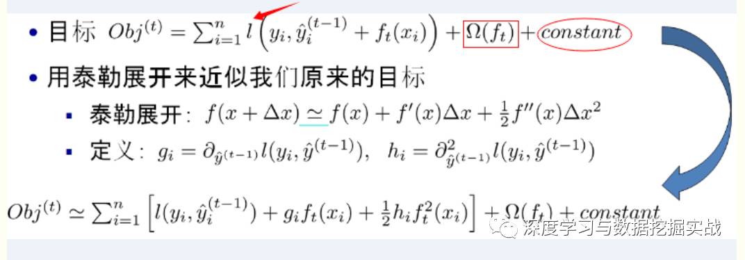
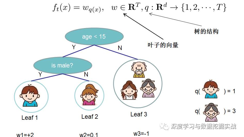
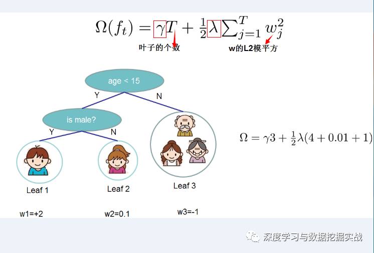
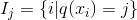
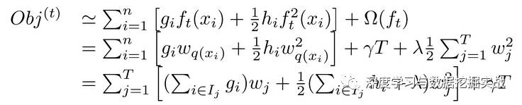
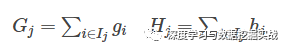
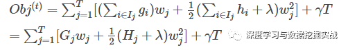
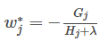
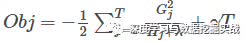
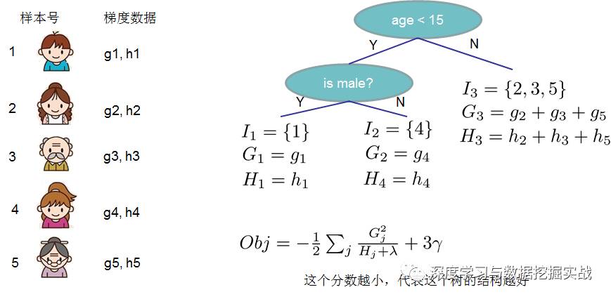
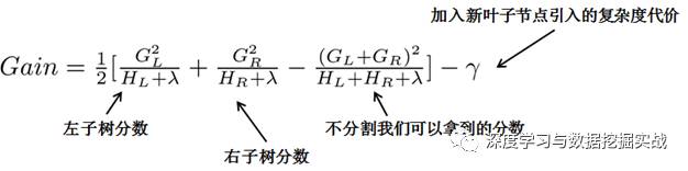
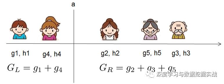
1, the background

On the principle of xgboost, there are very few resources on the network, and most of them still stay at the application level. This article hopes to understand the principle of xgboost by studying the PPT address and xgboost guide and actual address of Dr. Chen Tianqi.

2, xgboost vs gbdt

Speaking of xgboost, I have to say gbdt. Know gbdt can see the address of this article, gbdt is quite perfect in both theoretical derivation and application scenario practice, but there is a problem: the nth tree training needs to use the n-1th tree (approximate ) residual. From this point of view, gbdt is more difficult to achieve distributed (ps: although difficult, it is still possible, think about it from another angle), and xgboost starts from the following angle

Note: The red arrow points to the loss function; the red box is the regular term, including L1 and L2; the red circle is a constant term. Using Taylor to expand the three terms and make an approximation, we can clearly see that the final objective function depends only on the first and second derivatives of the error function of each data point.

3, the principle

(1) Defining the complexity of the tree For the definition of f, the tree is split into the structure part q and the leaf weight part w. The figure below is a concrete example. The structure function q maps the input to the index number of the leaf, and w gives the leaf score corresponding to each index number.

This goal consists of TT independent univariate quadratic functions. We can define

The final formula can be reduced to

Pass on

Then put

(2) Example of scoring function calculation

Obj represents the maximum amount we reduce on the target when we specify the structure of a tree. We can call it the structure score.

(3) greedy method of enumerating different tree structures

Greedy: Every time you try to add a split to an existing leaf

For each extension, we still have to enumerate all possible partitioning schemes. How to enumerate all partitions efficiently? I assume that we want to enumerate all the conditions such as x < a. For a particular split a we want to calculate the sum of the left and right derivatives.

We can see that for all a, we can enumerate all the gradients and GL and GR by doing a left-to-right scan. Then use the above formula to calculate the score for each split scheme.

Looking at this objective function, you will find that the second thing worth noting is that introducing a partition does not necessarily make the situation better, because we have a penalty that introduces a new leaf. Optimizing this target corresponds to the tree's pruning. When the introduced segmentation gain is less than a threshold, we can cut the segmentation. You can see that when we formally derive goals, strategies like calculating scores and pruning will naturally appear, rather than being manipulated because of heuristic.

4, custom loss function

In the actual business scenario, we often need a custom loss function. Here is an official link address

5, Xgboost adjustment

Due to the excessive number of Xgboost parameters, using GridSearch is particularly time consuming. Here you can learn this article and teach you how to step by step. address

6, python and R simple use of xgboost

Task: Two classifications, there is a sample imbalance problem (scale_pos_weight can interpret this problem to some extent)

7, the introduction of more important parameters in Xgboost

(1) Objective [ default=reg:linear ] Define the learning task and the corresponding learning objectives. The optional objective functions are as follows:

"reg:linear" – linear regression.

"reg:logistic" – logistic regression.

“binary:logistic” – The logistic regression problem for the two classifications, the output is the probability.

"binary: logitraw" – Logistic regression problem for the two classifications, the output is wTx.

“count:poisson” – Poisson regression for counting problems, the output is poisson distribution. In poisson regression, the default value of max_delta_step is 0.7. (used to safeguard optimization)

“multi:softmax” – Let XGBoost use the softmax objective function to handle multi-classification problems, and also need to set the parameter num_class (number of categories)

"multi:softprob" - Same as softmax, but the output is a vector of ndata * nclass, which can be reshaped into a matrix of ndata rows of nclass columns. No data indicates the probability that the sample belongs to each category.

"rank:pairwise" –set XGBoost to do ranking task by minimizing the pairwise loss

(2) 'eval_metric' The choices are listed below, evaluation indicators:

"rmse": root mean square error

"logloss": negative log-likelihood

"the error": Binary classification error rate. It is calculated as #(wrong cases)/#(all cases). For the predictions, the evaluation will regard the instances with prediction value larger than 0.5 as positive instances, and the others as negative Instances.

"merror": Multiclass classification error rate. It is calculated as #(wrong cases)/#(all cases).

"mlogloss": Multiclass logloss

"auc": Area under the curve for ranking evaluation.

“ndcg”: Normalized Discounted Cumulative Gain

"map":Mean average precision

"ndcg@n", "map@n": n can be assigned as an integer to cut off the top positions in the lists for evaluation.

"ndcg-", "map-", "ndcg@n-", "map@n-": In XGBoost, NDCG and MAP will evaluate the score of a list without any positive samples as 1. By adding "-" in The evaluation metric XGBoost will score these 0 as be consistent under some conditions.

(3) lambda [default=0] L2 regular penalty coefficient

(4)alpha [default=0] L1 regular penalty coefficient

(5) lambda_bias L2 regularity on the offset. The default value is 0 (there is no regularity for the offset term on L1, since the offset is not important at L1)

(6) eta [default=0.3] In order to prevent over-fitting, the shrinking step size used in the update process. After each lifting calculation, the algorithm directly obtains the weight of the new feature. Eta reduces the weight of features to make the calculation process more conservative. The default value is 0.3. The value range is: [0,1]

(7) max_depth [default=6] The maximum depth of the number. The default value is 6 and the value range is: [1, ∞]

(8) min_child_weight [default=1] The smallest sample weight sum in the child node. If the sample weight of a leaf node is less than min_child_weight then the splitting process ends. In the current regression model, this parameter refers to the minimum number of samples required to build each model. The larger the mature, the more conservative the value range of the algorithm is: [0, ∞]